The differential equations for the single pendulum and double pendulum can be solved exactly only in the harmonic approximation. Numerical methods can be used to solve the equations for any value of  and
and  .
.
The integration method used in this simulation is called the velocity Verlet algorithm. This algorithm is perhaps the most widely used algorithm for numerical integration of ordinary differential equation. First the (common) Verlet algorithm is discussed.
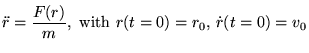
The Newton equation of motion for a particle of mass  subjected to a force
  is:
is:
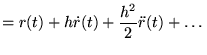
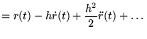
The Taylor approximations for  and
and  are :
are :
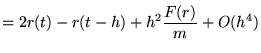
Adding (3) and (4):
and rearranging terms:
gives the Verlet algorithm.
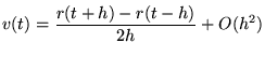
The velocity (
 ), if needed, can be calculated as:
 |
(6) |
Equation (6) has one drawback, it has an error  instead of the
  error of (5). If the velocity is important (for example for determining the kinetic energy to study energy conservation) the so called velocity Verlet algorithm is preferable.
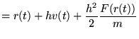
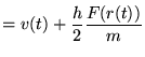
First and  are calculated from the forces at time
  :
:
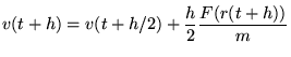
then the force at time  is calculated with this new position and used to calculate
 as:
as:
These equations are easily generalised to a system of interacting particles.
Velocity Verlet with adaptive stepsize
The step size should be chosen small enough to ensure energy conservation. To estimate a suitable stepsize, velocity Verlet with adaptive stepsize is used. It estimates the error of integration at every integration step and adjusts its stepsize accordingly.
In this simulation the algorithm is only used for one period of oscillation for a single pendulum. The smallest stepsize encountered by the adaptive stepsize algorithm will be used to perform the coupled pendulum simulation. The adaptive stepsize algorithm is derived as follows.
A simulation of a particle with mass subjected to a force starts at  with a known position
  . One integration step is done to approximate the position
 with an error , call this approximated position
  . The error of this integration step is defined:
Because the order of the error is  , taking half a stepsize results in an error approximately
  times smaller. Two steps are now needed to approximate , so the error is:
and also:
So an approximation of
 is found, at the cost of doing 2 extra steps of size
  .
.
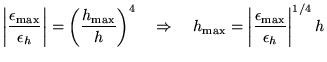
Define a maximum error
 for the simulation. Starting at one integration step of size
  is done to approximate
  . The position is also approximated by doing 2 steps of size . Both results are compared to get an estimate of
. With this error the maximum stepsize
. The position is also approximated by doing 2 steps of size . Both results are compared to get an estimate of
. With this error the maximum stepsize
 belonging to
is estimated:
belonging to
is estimated:
because of the of the error.
If
 , then is replaced by
 , and the integration is redone starting at . The new stepsize is multiplied by 0.9, to assure that the stepsize is always small enough.
If
 then the stepsize is small enough and the simulation proceeds to
  (where could have been changed by the previous step).
In most simulations the stepsize is also adusted when it is too small compared to
. It is not needed in this simulation because the algorithm is only used to find the smallest
. This ensures that the simulation with the two coupled pendula is performed with an error smaller than, or equal to
. Everytime parameters of the simulation are changed, the adaptive stepsize algorithm is used to estimate the stepsize.
The step size needed to meet the energy conservation condition is so small, that the simulation cannot be drawn at every step. About ten frames per second are drawn.